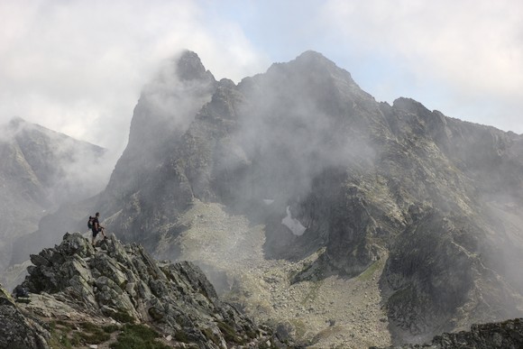
Die Hohe Tatra (Slowakei und Polen) ist ein winziges Hochgebirge, in dem zackige Granitberge mit hohen Wänden über unzähligen Bergseen aufragen. Vor einigen Jahren hatte ich in einer grandiosen dreitägigen Wanderung die Hohe Tatra von Nord nach Süd durchquert, musste dann aber aus familiären Gründen den Trek abbrechen. Was ich damals — insbesondere auf slowakischer Seite — verpasst habe, wollte ich dieses Jahr nachholen. Rund eine Woche reicht aus, um nahezu jedes Hochtal zu erkunden.
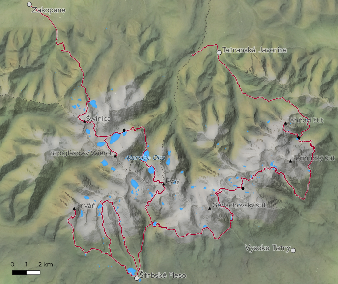
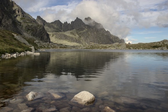
Ich reiste per Zug nach Zakopane (Polen) an und nahm dann morgens einen Minibus (Richtung Morskie Oko) bis zum Grenzübergang Lysá Pol’ana. Nach einem kurzen Stück auf der Straße bog ich in Tatranská Javorina in das Tal ab, das die Hohe Tatra von der Belaer Tatra trennt, und stieg bei Nebel und Regenschauern zum Pass Kopské sedlo auf. Das Wetter wurde zum Glück genau in dem Moment besser, als ich oben ankam und ein Stück weiter in einen weiten Talkessel wechselte, an der westlichsten Ecke der Hohen Tatra. Wenig später erreiche ich die in einem spektakulären Talabschluss an einem See gelegene Hütte Chata pri Zelenom plese. Am späten Nachmittag besteige ich noch den Aussichtsberg Jahňací štít: direkt neben mir die hohe Granitwand des Lomnický štít, rechts im Hintergrund reicht der Blick bis Rysy, Kriváň und Świnica (und damit bis ans andere Ende des kleinen Gebirges). Und auf der anderen Seite die Kalkberge der Belaer Tatra.
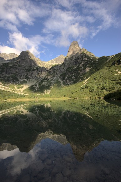
See bei der Chata pri Zelenom plese
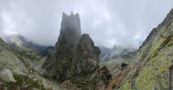
Nach einem stimmungsvollen Morgen am See steige ich auf der Tatra-Magistrale (einem klassischen Fernwanderweg, der auf mittlerer Höhe am Rand des Gebirges entlangführt) den benachbarten Rücken auf, stecke dort allerdings wieder im Nebel. Es geht, wieder unterhalb der Wolken, zu einer von Touristen umwuselten Seilbahnstation und, immer leicht absteigend am Hang entlang, weiter zum nächsten Taleingang. Hier zweige ich von der Tatra-Magistrale ab und steige durch das Tal Mala Studena dolina auf. Am Nachmittag sitze ich an einem der Seen im Talkessel, bevor ich in leichter Kraxelei über die Scharte Priečne sedlo ins benachbarte Tal Velka Studena dolina wechsle. An weiteren, im oberen Ende dieses Tals verstreuten Seen vorbei erreiche ich die Hütte Zbojnicka chata.
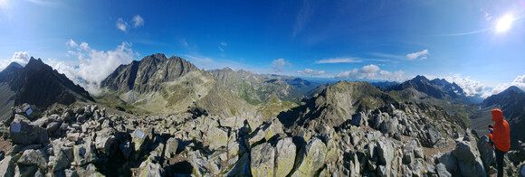
Da der Wetterbericht mir nur noch einen guten Tag verspricht, breche ich früh morgens auf und steige zur Prielom-Scharte auf. Hier öffnet sich — durch die Felsen etwas eingeschränkt — der Blick auf den Gerlach, den höchsten Berg der Tatra. Es geht ein wenig in das Tal auf der Nordseite des Gebirges abwärts und gleich wieder zum nächsten Pass hinauf. Von hier steige ich auf den Aussichtsberg Východná Vysoká auf, mit großartiger Rundumsicht.
Východná Vysoká (360°-Panorama)
Es geht das Tal abwärts bis zu einem an einem See gelegenen Berghotel, ab dem ich wieder auf die Tatra-Magistrale treffe. Auf dieser geht es zu einem weiteren, auf der Südseite des Gerlach gelegenen Sees, und weiter bis zu einem weiteren guten Aussichtspunkt, Ostrva, einem Bergrücken hoch über dem See Popradské pleso. Zu diesem steige ich ab, und wandere noch bis Štrbské Pleso, einem ebenfalls an einem See gelegenen, aber nicht allzu hübschen Ferienort. Da hier die Preise vergleichsweise hoch sind, nutze ich die Zahnradbahn und komme am Fuß des Gebirges in Štrba unter.
Blick von Ostrva über den See Popradské pleso
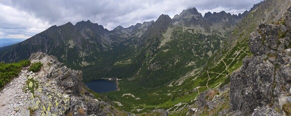
Den Tag mit dem schlechtesten Wetter verbringe ich in der Stadt Poprad. Eine Tageswanderung führt mich von Štrbské Pleso auf den Kriváň, aber außer Wolken und Nebel ist leider nichts zu sehen. Etwas mehr Glück habe ich bei einer weiteren Wanderung durch die beiden oberhalb von Štrbské Pleso gelegenen Hochtäler, über die Scharte Bystrá lávka.
Hochtal Furkotská dolina und Krivan von der Scharte Bystrá lávka
Am ersten Tag mit richtig gutem Wetter nehme ich eine der ersten Bahnen — vor Sonnenaufgang — nach Štrbské Pleso, wandere wieder beim Popradské pleso vorbei und steige zum Rysy auf. Ich war allerdings nicht der einzige, der sich früh auf den Weg gemacht hat. An einer Steilstufe mit Leiter hat sich schon ein regelrechter Stau gebildet, und auf dem für seine grandiose Aussicht berühmten Doppelgipfel musste ich mich durch die Menschenmassen zwängen, um ein noch freies Plätzchen zu erreichen.
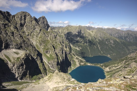
Auf der polnischen Seite stieg ich wieder ab, wobei ich meist etwas abseits der Ketten über die steilen Felsplatten abstieg, während neben mir immer mehr Menschen aufwärts hangelten. An einem besonders schönen Aussichtspunkt auf halber Höhe machte ich eine lange Mittagspause, unter mir die Seen Czarny Staw pod Rysami und Morskie Oko (Meerauge). Als ich später an den Seen ankam, war dort ein derartiger Trubel, dass ich mich beeilte, weiterzukommen. Ich stieg noch ins Fünfseental auf und übernachtete in der dortigen Hütte.
Czarny Staw pod Rysami und Morskie Oko
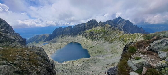
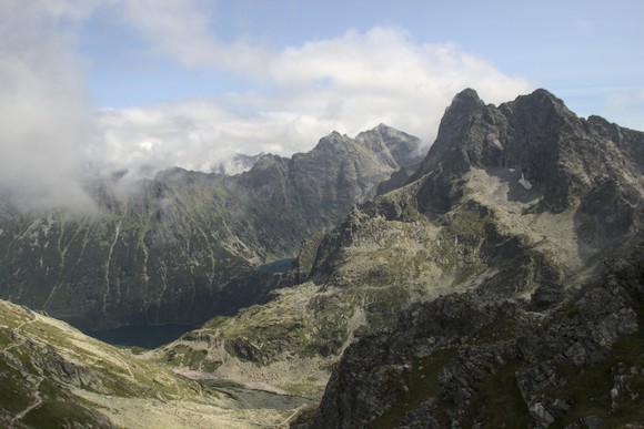
Es folgte ein weiteres Zwischentief, mit strömendem Regen am Morgen. Kurzerhand beschloss ich, eine weitere Nacht zu bleiben und das Tal zu erkunden. Als es etwas besser wurde, stieg ich zum Aussichtsberg Szpiglasowa Przełęcz, auf dem ich genau den richtigen Moment erwische: Für kurze Zeit reißt es auf und gibt den Blick auf all die Seen und Berge der Umgebung frei — wenige Stunden später verschwinden die Berge wieder in Wolken.
Blick von Szpiglasowa Przełęcz
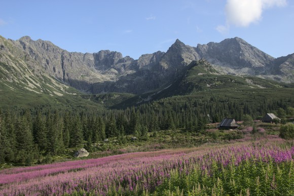
Endlich beginnt eine Hochwetterlage, was aber auch einen erheblichen Nachteil hat: Über die Wanderwege wälzen sich Menschenmassen, die Hütten sind überfüllt und selbst in Zakopane kann ich keine günstige Unterkunft mehr buchen. Ich steige auf den Gipfel des Świnica auf, der die Nordwestecke der Hohen Tatra bildet, schlage einen Bogen über den See Zielony Staw Gąsienicowy nach Hala Gąsienicowa Rówienki, wo es ein paar hübsche Holzhäuser mit Bergen im Hintergrund gibt. Mit Aussichten auf den Giewont erreiche ich Kuznice, von wo ich das letzte Stück die Straße entlang bis Zakopane gehe.
In QGIS wird eine NetCDF-Datei als Raster mit einem Band pro Zeitstempel geöffnet. In den Temporal Settings wird die Zeit leider nicht eingestellt, aber sie steht im Namen des Bands und kann mit einer Expression umgewandelt werden
Wenn ich eine NetCDF-Datei in QGIS als Raster öffne, dann bekomme ich ein Rasterlayer mit sehr vielen Bändern, ein Band pro Zeitstempel. Leider werden beim Öffnen die zeitlichen Einstellungen dieser Bänder nicht eingestellt, sodass man nicht einfach mit der Zeitsteuerung einzelne Zeitpunkte wählen oder eine Animation abspielen kann. Immerhin steht der Zeitstempel im Namen des Bands, allerdings in der Form time=1867128 (hours since 1800-01-01). Das reicht zum Glück aus, um in den Layereigenschaften unter „Zeitlich“ Anfang und Ende mithilfe einer Expression einzutragen (unter Konfiguration: „Fester Zeitraum je Kanal“).
Für den Anfang:
-- Epoche extrahieren und zu datetime umwandeln
to_datetime(
  right(
    regexp_substr(@band_name, 'hours since \\d{4}-\\d{2}-\\d{2}')
  , 10)
)
-- Anzahl der Stunden hinzuaddieren
+
make_interval(
  hours:=to_int(
	regexp_substr(regexp_substr(@band_name, 'time=\\d+'), '\\d+')
))
Jetzt kann man aus der Tabelle ablesen, wie groß die Zeitschritte sind (z.B. 6 Stunden). Für „Ende“ können wir das entsprechende Intervall zu obiger Expression hinzuaddieren:
-- Vollständige Expression von oben
+ make_interval(hours:=6)
Visualisierung von saisonalen oder zyklischen Zeitreihendaten als kreisrunde Heatmap in Polarkoordinaten
Mir gefällt, wie die Datenuhr in ArcGIS Pro saisonale Muster in Zeitreihen visualisiert. Die Ringe des Diagramms zeigen die größere, zyklische Zeiteinheit (z. B. das Jahr), während jeder Ring in kleinere Einheiten unterteilt ist, die als Keile dargestellt werden. Natürlich wollte ich dasselbe mit Open-Source-Tools machen können, und das war in Python mit Pandas und Plotly möglich.
Mit meinem QGIS-Plugin Data Clock kann das Diagramm direkt aus der Processing-Toolbox erstellt werden, und zwar mit jedem Vektorlayer, das mindestens ein Date- oder DateTime-Feld enthält. Es ist auch möglich, die Funktionen der figure factory von der QGIS-Python-Konsole aus aufzurufen. Die Features werden auf diese Ringe und Keile verteilt und die Farbe wird durch die Anzahl der Features oder durch eine Aggregationsfunktion (z.B. Summe, Mittelwert, Median) auf einer bestimmten numerischen Spalte bestimmt. Die folgenden Kombinationen von Ringen und Keilen sind implementiert: Jahr-Monat, Jahr-Woche, Jahr-Tag, Woche-Tag, Tag-Stunde. Das Ergebnis ist eine HTML-Datei mit einem interaktiven Plotly-Diagramm (einschließlich eines Tooltips).
Das Plugin befindet sich in der QGIS Plugin Registry und kann in QGIS über „Erweiterungen“ – „Erweiterungen verwalten und installieren“ installiert werden. In den Einstellungen muss der Haken bei „Experimentelle Plugins anzeigen“ gesetzt sein. Plotly und Pandas müssen installiert sein.
Datenuhr in Python
Wer diese Art von Diagramm in Python mit Plotly und Pandas erstellen möchte, kann einen Blick in mein Jupyter Notebook werfen.
Plotly in der QGIS Python Console verwenden
Es ist ziemlich einfach, Plotly für jede Art von Diagrammen aus den Daten eines Vektorlayers zu verwenden, direkt von der QGIS Python-Konsole aus. Dabei ist zu beachten, dass die High-Level-Funktionen von Plotly Express Daten in einem Pandas DataFrame erwarten, daher ist es besser, die Plotly Graph Objects direkt zu verwenden. Der folgende Code holt die Daten von zwei Feldern mithilfe einer List Comprehension, erstellt ein Scatter Plot und fig.show() öffnet das Diagramm in einem Browser. Auf diese Weise kann man auf Plotly-Methoden wie update_layout(), update_traces() oder to_html() zurückgreifen.
import numpy as np
import plotly.graph_objects as go

layer = iface.activeLayer()

x_field = 'dateofocc'
y_field = 'victim_l'

x = [f[x_field] for f in layer.getFeatures()]
y = [f[y_field] for f in layer.getFeatures()]

fig = go.Figure(
    layout_title_text="Title"
)

fig.add_trace(go.Scatter(
    x=x,
    y=y,
    mode='markers'
))

fig.show()
Mit dem Plugin Adjust Style kann eine Schriftart überall in der Karte durch eine andere ersetzt werden
Die in einer Karte verwendeten Schriftarten tragen einiges zum Erscheinungsbild einer Karte bei. In der Regel verwendet man dieselbe Schriftart an vielen Stellen: etwa im Titel, im Impressum, in der Legende und dem Maßstab, vielleicht auch für Labels in der Karte selbst. Oft stellt man sich die Frage, ob nicht diese oder jene Schrift besser aussehen würde. Bisher musste man in QGIS im Print-Layout die Schrift an vielen Stellen ändern, um das auszuprobieren. Das ist mühsam und braucht so viel Zeit, dass man nur ungern mit verschiedenen Schriftarten experimentiert.
Mit meinem QGIS-Plugin Adjust Style ist das nun (seit Version 1.9) mit wenigen Klicks möglich: Einfach im Print-Layout-Fenster das Plugin öffnen, „Replace Font“ wählen, die alte (zu ersetzende) und die neue Schriftart wählen und OK klicken. Mit Checkboxen kann man auch feiner einstellen, wo überall die Schrift geändert werden soll. Um die Schrift von Labels in der Karte selbst zu ändern, muss man dasselbe (wie in den alten Versionen des Plugins) im Hauptfenster (mit entsprechend gewählten Layern) machen.
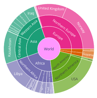
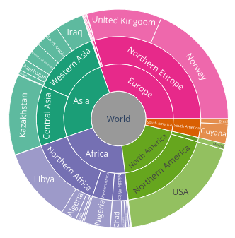
Ein einfacher Hack zum Ändern der Farbe in der Mitte eines Sunburst-Diagramms
Ich habe einen Datensatz mit vielen Zeilen pro Land als sunburst chart mit Plotly dargestellt. Da ich aus dem Natural Earth Dataset die countries in meinen Pandas dataframe gejoint habe, hatte ich auch die Spalten ‚CONTINENT‘ und ‚SUBREGION‘. Ich konnte also einfach einen Plot erstellen mit:
Allerdings änderten sich nun die Farben in einem mit Dash erstellten Dashboard je nach angewandtem Filter. Ich musste also feste Farben für die Kontinente verwenden, etwa so:
# Dictionary mit Farben für jeden Kontinent
cat_colors={}
for i, continent in enumerate(countries["CONTINENT"].unique()):
    cat_colors[continent] = px.colors.qualitative.Dark2[i]

fig = px.sunburst(
    df,
    path=[px.Constant("World"), 'CONTINENT', 'SUBREGION', 'country'],
    values='Qty',
    color_discrete_map=cat_colors,
    color='CONTINENT',
    )
Leider gibt es keine Möglichkeit, die Farbe von „World“ im Zentrum des Diagramms an dieser Stelle einzustellen, sie erhält einfach eine zufällige Farbe (und in meinem Dashboard änderte sich die Farbe je nach Filter). Ich konnte keine Lösung im Internet finden, selbst ChatGPT konnte nicht weiterhelfen. Nach langer Zeit erinnerte ich mich daran, dass Plotly-Fig-Objekte im Grunde JSON sind; es ist einfach, die JSON-Daten zu inspizieren und sie anschließend zu ändern. Um die Farbe von „World“ auf Grau zu setzen, reichen folgende Zeilen:
RasterWizard: Daten eines QGIS Rasterlayers als Numpy-Array in der Python-Konsole – und das Ergebnis zurück in QGIS
Die neueste Version meines QGIS-Plugins SciPy-Filter enthält RasterWizard, eine Hilfsklasse für Python-Benutzer, um schnell die Daten eines Raster-Layers als NumPy-Array und das Verarbeitungsergebnis zurück in QGIS als neuen Raster-Layer zu erhalten. Dies ermöglicht die Verarbeitung mit NumPy, SciPy, scikit-image, scikit-learn oder anderen Python-Bibliotheken – und die sofortige Visualisierung der Ergebnisse in QGIS. Dies ist ideal für die Entwicklung von Prototypen und das Experimentieren mit Algorithmen.
Einfach in QGIS die Python-Konsole öffnen und etwas ausführen wie:
from scipy_filters.helpers import RasterWizard
from scipy import ndimage

wizard = RasterWizard() # Verwendet das aktive Layer, wenn kein Layer gegeben
a = wizard.toarray()    # Gibt NumPy-Array mit allen Bändern zurück

# Irgendeine Berechnung, z.B. Sobel-Filter mit Scipy
# In diesem Beispiel ist das Ergebnis ein NumPy-Array mit dtype float32
b = ndimage.sobel(a, output="float32")

# Ergebnis als geotiff speichern und in QGIS laden
wizard.tolayer(b, name="Sobel", filename="/path/to/sobel.tif")
Das NumPy-Array hat die Dimensionen [Bänder], x, y. Man kann also ein Band mit z.B. a[0] auswählen. Mit der Option bands_last=True bekommt man stattdessen x, y, [Bänder], wie es scikit-image erwartet.
Das resultierende NumPy-Array kann als neuer Rasterlayer zurück in QGIS geladen werden, solange die Anzahl der Pixel die gleiche ist wie die des Eingangslayers und die Geotransformation nicht verändert wird (keine Reprojektion, kein Subsetting in NumPy). Die Anzahl der Bänder und der Datentyp können unterschiedlich sein.
Weitere Infos über das Raster:
# Pixelwerte an Index [x, y]
wizard[0,10]

# Informationen wie shape, CRS, usw.
wizard.shape   # wie numpy_array.shape
wizard.crs_wkt # CRS als WKT string
wizard.crs     # CRS als QgsCoordinateReferenceSystem
Das Plugin kann in QGIS mit „Erweiterungen verwalten und installieren“ installiert werden. Für weitere Informationen siehe die API-Dokumentation für RasterWizard.
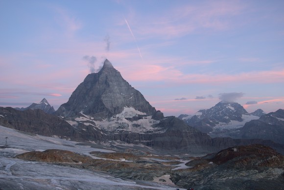
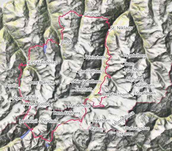
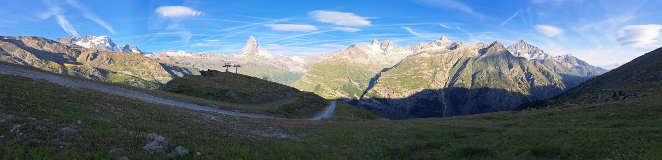
9-tägige Trekking-Runde um Matterhorn, Weisshorn und Dent Blanche
Matterhorn, Aussicht nahe Gandegghütte
Das Matterhorn ist nur der bekannteste Berg, um den der 9-tägige Trek herumführt, und es ist nur auf etwa 1/3 der Stecke zu sehen. Man wandert auch um eine Reihe weiterer beeindruckender 4000er herum: Weisshorn, Zinalrothorn, Obergabelhorn, Dent Blanche und Dent d’Hérens. Flankiert wird die Route von Monte Rosa, Breithorn, Dom und den anderen Gipfeln der Mischabel. Während man die meisten Postkartenansichten rund um Zermatt bekommt, gefallen mir gerade die abgelegenen und weniger überlaufenden Täler entlang der Route, etwa das Turmanntal und die Pässe Col Collon und Col de Valcournera. Man muss dazusagen, dass man (auch laut Führer) mehrmals auf Seibahnen zurückgreift, die Umrundung also nicht ganz zu Fuß ist.
Ich parke in St. Niklaus, das im Mattertal an der Straße Richtung Zermatt liegt, und starte früh morgens mit der ersten Seilbahn auf die Alp Jungu. Am Vorabend fuhr ich im Schritttempo durch ein heftiges Gewitter, dafür sah es jetzt ganz OK aus: zwar einige Wolken, aber ein toller Blick über die Alp hinweg das Mattertal aufwärts, zwischen Mischabel und Weisshorn hindurch auf das im Morgenlicht leuchtende Breithorn. Aber für den späten Mittag war das nächste Unwetter angekündigt, daher gab ich Gas. Schon wenig später bekomme ich den ersten Schauer ab, und während ich auf dem Augsbordpass verschnaufe rollt über den Bergrücken auf der anderen Seite des Turtmanntals eine schwarze Wand, in der Blitze zucken. So früh hatte ich damit nicht gerechnet. Ich steige noch ein Stück ins Tal ab und baue dann in strömenden Regen und Hagel mein Zelt auf, damit ich an einem trockenen und warmen Ort auf besseres Wetter warten kann. Das kommt dann aber schneller als gedacht und am Mittag bin ich bei strahlender Sonne im Dorf Gruben-Meiden im Turtmanntal.
Auf der anderen Talseite steige ich wieder auf, und während ich die Alp Meide passiere, braut sich bereits das nächste Gewitter zusammen. Diesmal finde ich rechtzeitig einen guten Ort, um mein Zelt aufzubauen.
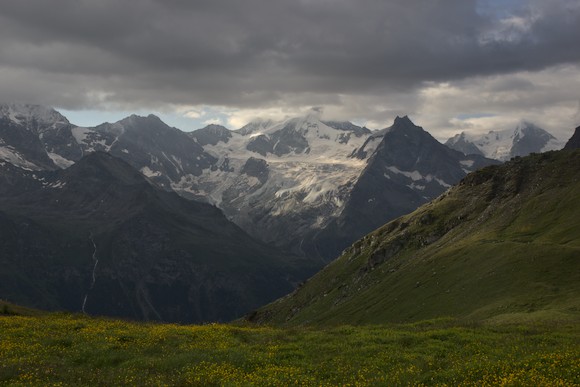
Am Morgen wieder strahlende Sonne. Es geht über den Meidpass und vorbei am Hôtel du Weisshorn, dann auf einem Höhenweg hoch über dem Tal bis Zinal. Leider stecken die hohen Gipfel am Talschluss, wie Zinalrothorn, Obergabelhorn und Dent Blanche, schon wieder in Wolken.
Blick von Sorebois
In Zinal stocke ich die Vorräte auf und nehme noch die Seilbahn nach Sorebois (die letzte fährt schon um 16 Uhr!), wo ich am Rand des Skigebiets eine flache grasige Stelle finde, an der es einen halbwegs unverdrahteten Ausblick gibt. Die Berge stecken zwar in Wolken, aber ich hoffe auf einen schönen Morgen. Als ich aufstehe ist das Wetter leider nicht viel besser. Über eine Skipiste steige ich zum Col de Sorebois auf und blicke auf den türkisgrünen Stausee Lac de Moiry hinab — bis ich wenig später in einer Wolke stecke. Zur Staumauer steige ich nun ab, hin und wieder ist in einer Wolkenlücke Dent Blanche oder einer seiner Nebengipfel zu sehen. Unten scheint wieder die Sonne, ich überschreite die Dammkrone und steige auf der anderen Seite zum kleinen Lac des Autannes auf, der gerade noch unterhalb der Wolken liegt, die penetrant am Bergrücken hängen. Entsprechend geht es mit wenig Sicht über den Col de Torrent hinüber ins Val d’Hérens. Wieder bei Sonne geht es über Almwiesen hinweg abwärts, dann von Dorf zu Dorf zum Talboden in Les Haudères. Das Tal verzweigt sich an dieser Stelle, das linke Tal führt steil zu einem Gletscherplateau hinauf, neben bzw. hinter dem je nach Blickrichtung Dent Blanche oder Dent d’Hérens zu sehen sind. Im anderen Tal liegt etwas höher Arolla, darüber ragen die Pigne d’Arolla (übrigens ein toller Skitourenberg mit beidruckendem Blick auf die Westseite des Matterhorns) und der Mont Collon auf, auf dessen Rückseite dieser Trek über einen Pass nach Italien führt.
Um nach Arolla zu kommen, steigt die Route von Les Haudères steil zur Alm Mayens de la Couta und noch ein gutes Stück weiter auf, noch mit schönen Blicken. Hier oben fällt es mir schwer, einen guten Platz zum Biwakieren zu finden, zumal mir ganz oben eine riesige Kuhherde auf dem Weg zum Melken entgegen kommt. Dann geht es relativ eintönig in stetigem auf und ab nahezu hangparellel durch lichten Wald nach Arolla, was ich sehr anstrengend finde, vor allem weil ich nicht durch Ausblicke entschädigt werde. Einzige Ausnahme ist der durchaus hübsche Bergsee Lac Blanc.
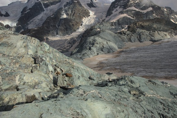
Etwas oberhalb von Arolla, am Ende des Sträßchens, ist der Wanderweg gesperrt, weil eine Brücke über eine in die Moräne geschnittene Schlucht zerstört ist. Erstmal ein Schock, weil das auf der Karte die einzige Möglichkeit ist, um in das Hochtal (und damit Richtung Italien) zu kommen. Zum Glück kann man (mühsam) über die Winterroute ausweichen. So sitze ich Mittags gegenüber des Gletscherabbruchs neben dem Mont Collon und staune darüber, dass auf dem Felsgrat daneben die Cabagne des Vignettes trohnt, in der ich mal eine Sturmnacht verbracht habe. Am Abend steige ich über den Haut Glacier d’Arolla auf (der deutlich kürzer als auf der Karte und den Fotos im Führer ist und auch nicht so weiß, so viele Felsblöcke sind aus dem schmelzenden Eis freigesetzt worden), und kraxle hinter dem Mont Collon noch die Seitenmoräne hinauf, wo ich mit Blick auf den Gletscher zelte.
Haut Glacier d’Arolla
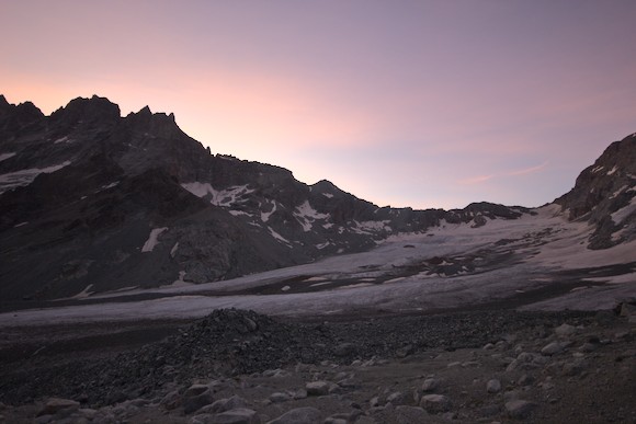
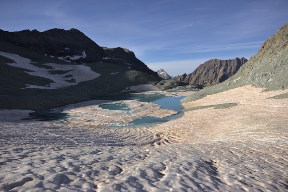
Früh morgens steige ich das letzte Stück zum Pass Col Collon auf, wieder über einen Gletscher, der von dem großen Gletscherplateau hinab kommt. Der Pass ist wunderschön, mit einem Schmelzwassersee auf der italienischen Seite, in dem Eisschollen schwimmen.
Col Collon
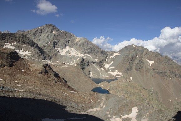
Nun geht es in eine von Felsen geprägte Bergwelt abwärts, bis ans hintere Ende eines Stausees, und auf der anderen Seite wieder hinauf in ein anderes Hochtal. Aus diesem heraus führt ein schweißtreibender Anstieg über zwei Steilstufen zum Col de Valcournera. Auf der anderen Seite sind wenig unterhalb ein paar Bergseen und eine Hütte zu sehen. Ich steige bis zur oberhalb des Lac Balanselmo liegenden Biwakschachtel ab, wo ich einen guten Platz für mein Zelt finde. Es war wohl die Lieblingswiese eines Steinbocks, jedenfalls graste dieser den ganzen Abend über friedlich neben meinem Zelt.
Col de Valcournera
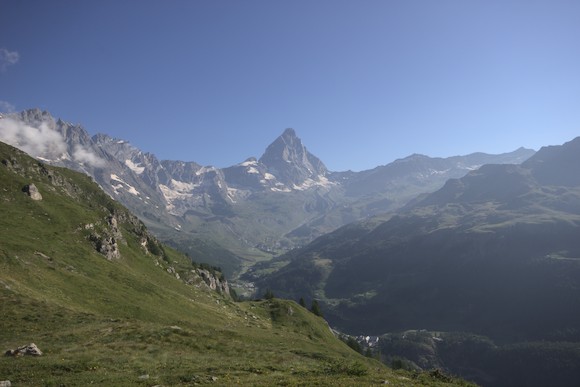
Am morgen geht es weiter abwärts und wird immer grasiger. Nach einem kurzen Gegenanstieg und einer weiteren Kurve steht man unmittelbar der Südwand des Matterhorns gegenüber, oder besser gesagt: Cervinia. Auf diesen Bergzacken laufe ich noch eine Weile auf einem hochgelegenen Weg zu, bis es auf den Talboden hinabgeht.
Matterhorn (Cervinia)
Leider sind die Spazierwege auf beiden Seiten des Flusses gesperrt (der eine wegen fliegenden Golfbällen), aber ich finde eine Alternativroute oberhalb der Straße, die mich in den Ort Breuil-Cervinia bringt. Dort streife ich durch alle möglichen kleinen Läden, um den Proviant aufzufüllen, der Supermarkt ist so verrammelt, als ob er nie wieder aufmacht und die kleinen Läden haben nur eine kleine Auswahl. Endlich fahre ich mit der Seilbahn nach Plan Maison ins Skigebiet, wo es leider im Sommer ziemlich furchbar aussieht. Über die Narben des Wintersports wandere ich aufwärts (über die Piste rumpeln immer wieder Pickups auf und ab) und erreiche schließlich den höchsten Punkt des Treks, den Theodulpass. Das ist allerdings wieder ein Schock, weil die ganze Umgebung der Hütte gerade eine große Baustelle ist. Zwei Bagger und anderes schweres Gerät wühlen sich gerade durch das Gestein und bauen die Piste um. Ich frage erstmal in der Hütte, bevor ich mich am Verbotsschild vorbeitraue, am Bagger vorbei (der Baggerführer winkt mir zu) und dann durch die Mischung aus Schlamm, Fels- und Eisbrocken, in die der Bagger die Piste verwandelt hat. Über einen steilen Hang aus Schutt und Eis geht es auf den Theodulgletscher, über den ich im Abendlicht einer Piste folgend absteige.
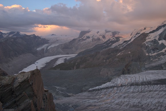
Meine Laune wird wieder besser: Das in einer Wolke steckende Matterhorn wird hin und wieder schemenhaft sichtbar, die grünen Rundhöcker aus Grünstein und Serpentinit leuchten im Abendlicht (siehe auch mein Buch Bewegte Bergwelt: Gebirge und wie sie entstehen mit einem Abschnitt über die Geologie Rund um Zermatt). Und einige der anderen 4000er, die Zermatt umgeben, sind nahezu wolkenfrei. Allerdings ist deutlich zu sehen, dass es den Gletschern nicht gut geht. Ich war vor ca. 20 Jahren zum letzten Mal in Zermatt und damals gab es deutlich mehr Weiß in der Landschaft. Ich überlege, wo ich übernachten kann, um bei Sonnenauf- und untergang einen freien, möglichst wenig von Seilbahnen gestörten Blick zu haben. Schließlich baue ich mein Zelt nahe der Gandegghütte direkt unter der Seilbahn auf und werde mit tollen Fotos belohnt.
Kurz nach Sonnenaufgang zieht es wieder zu, während auf den Gletschern im Osten (Cima di Jazzi) noch Sonnenflecken scheinen und über mir die Seilbahn sich in Bewegung setzt. Während ich ins Tal absteige, scheint aber zum Glück die Sonne wieder, nur die höchsten Berge bleiben eingehüllt. Furi, ein hochgelegener Ortsteil von Zermatt, ist heute mein tiefster Punkt. Der Führer schickt mich über einen Waldweg Richtung Grünsee, aber ich will noch ein bisschen was sehen und nehme die Seilbahn auf den Riffelberg, um über den Panoramaweg zum Gornergrad hinauf zu steigen. Mir kommen dort massenhaft Touristen entgegen, die alle diesen Weg hinab laufen…
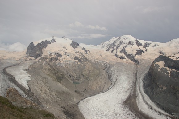
Während ich gerade noch in der Sonne lag und dann nahe Riffelsee auf den Gletscher hinab geblickt habe, donnert es hinter mir: Der Himmel im Westen hat sich in eine schwarze Wand verwandelt und mir bleibt gerade noch genug Zeit, um meine Regensachen anzuziehen. Kurz entschlossen steige ich bis zu einer nahe gelegenen Skilift-Bergstation auf und stelle mich dort unter, und wieder einmal dauert es nicht lange bis wieder ein Stückchen blauer Himmel zu sehen ist. Später sitze ich auf der Aussichtsplattform am Gornergrad, langsam schälen sich Monte Rosa und Trabanten aus ihrer Wolkenhülle. Der Himmel bleibt weitgehend bedeckt, aber die Berge leuchten in einem merkwürdigen indirekten Licht.
Monte Rosa und Lyskamm vom Gornergrad
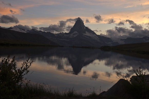
Schließlich geht es hinunter zum Grünsee und auf der anderen Seite hinauf zum Stellisee, wo ich gerade rechtzeitig zum Sonnenuntergang ankomme. Dass dies einer der besten Fotospots für das Matterhorn ist, ist kein Geheimnis: Sowohl bei Sonnenauf- und untergang drängen sich Touristen und Fotografen am Ufer. Und am besten Spot ist das Wasser voller Algen…
Matterhorn vom Stellisee
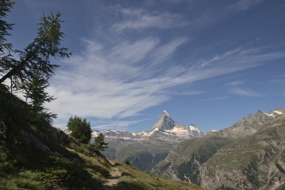
Am Morgen wandere ich über Blauherd nach Sunnega, wo der Europaweg beginnt: Dieser Höhenweg bildet die letzten zwei Etappen der Tour Matterhorn, und er bietet grandiose Ausblicke auf Matterhorn und Weißhorn. Weite Strecken sind so schön, dass man vor Lauter Fotos schießen nur langsam voran kommt. An der Täschalm kommen plötzlich auch Dom, Täschorn und Rimpfischhorn in Blick.
Breithorn, Matterhorn, Obergabelhorn, Zinalrothorn, Weisshorn von Blauherd
Bei einer Querung eines steinschlaggefährdeten Hangs geht es durch Lawinengallerien und kurze Tunnels. Die Anlagen haben schon einiges abbekommen, bei den Gallerien ist hin und wieder der Stahlbeton der Decke zerborsten und ein Tunnel ist von einer Mure so weit verfüllt, dass es mit Rucksack mühsam ist, sich hindurchzuzwängen.
Europaweg
Der übernächste Taleinschnitt ist wieder ein Steinschlaghang, auf dem immer wieder große Blöcke herunterpurzeln. Aber man wandert einfach auf der längsten Fußgängerhängebrücke der Welt darüber hinweg. Wenig später erreicht man die Europahütte und etwas weiter finde ich am Miesboden einen schönen Platz zum biwakieren.
Der letzte Tag ist dann leider enttäuschend. Der ursprüngliche Europaweg führte von hier stetig aufwärts auf einen Aussichtsberg, an dem sich der Blick auf die Berner Alpen öffnen würde. Dann ging es hinab nach Grächen, einem Ort oberhalb von St. Niklaus. Die Strecke ist aber seit einigen Jahren gesperrt und der neue Europaweg führt abwärts und erreicht bei Herbriggen den Talboden. Statt nun im Wald nach Grächen hinaufzuwandern bleibe ich im Tal. Es sind nur noch 2,5 km zum Auto.
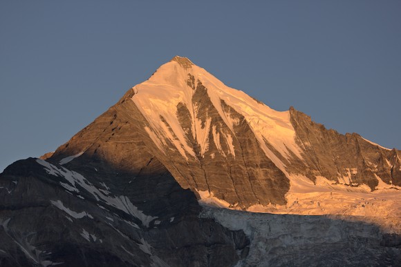
Weisshorn
Es war ein sehr schöner Trek, auf jeden Fall in einer Liga mit der Tour du Mont Blanc und den Dolomiten-Höhenwegen. Und das Matterhorn ist ja schon ein besonderer Berg. Ich würde es nicht als den schönsten der Welt bezeichnen, weil es da einige weitere Kandidaten gibt (z. B. Ama Dablam, Cerro Torre, Alpamayo, Cotopaxi, Mayon), aber es ist auf jeden Fall einer der markantesten. Und die Geologie der Gegend ist besonders spannend (siehe mein Buch Bewegte Bergwelt). Erstaunlicherweise habe ich kaum Leute getroffen, die die selbe Runde gemacht haben.
Die quadratische Alternative zu Kuchendiagrammen mit Plotly und Python erstellen
Nachdem ich gelernt habe, Waffle Charts in Tableau zu erstellen, wollte ich das auch in Python mit Plotly machen. Allerdings habe ich im Netz kein Beispiel gefunden, wo das Ergebnis meiner Vorstellung entsprach. Ein Waffle Chart ist quasi eine quadratische Alternative zu Kuchendiagrammen: es besteht aus 100 kleinen farbigen Quadraten in einem 10×10 Gitter.
In einem Jupyter Notebook erkläre ich, wie ein Waffle Chart mit Plotly erstellt werden kann.
In QGIS ignorieren Filter normalerweise Zellen mit No Data automatisch. Allerdings ist das nicht immer einfach, insbesondere wenn ein Filter benachbarte Zellen untersucht und diese No Data enthalten. Was dann passiert, hängt von der Implementierung ab, ist aber in beiden Fällen problematisch.
Zunächst ist „No Data“ in Rasterlayern mit einer bestimmten Zahl codiert, z.B. -9999. Wenn jetzt z.B. der Mittelwert innerhalb einer 3✕3-Nachbarschaft berechnet wird, kommt in der Umgebung jeder No-Data-Zelle natürlich Blödsinn heraus. Ersetzt man (in Numpy) die -9999 mit NaN (was es nur bei float gibt), führt das bei vielen Algorithmen dazu, dass die betreffende Zelle nun ebenfalls No Data wird, weil eine Berechnung nicht möglich ist. Die No-Data-Zellen stecken sozusagen ihre Nachbarschaft an.
Eine Möglichkeit ist, die No-Data-Zellen mit irgendeinem halbwegs sinnvollen Wert zu füllen. Dafür gibt es sowohl von QGIS selbst als auch über GDAL verschiedene Möglichkeiten, die allerdings den Nachteil haben, dass immer nur ein einziges Band verarbeitet wird. Man müsste also jedes Band einzeln verarbeiten und dann die Ergebnisse wieder zu einem Layer zusammenführen.
Dem Mittelwert des Bands (von GDAL geschätzt oder exakt berechnet)
Dem Minimalwert des Datentyps
Dem Maximalwert des Datentyps
Dem zentralen Wert des Datentyps
Später will man wahrscheinlich wissen, welche Zellen ursprünglich „No Data“ waren. Das Plugin kann auch eine No-Data-Maske (binäres Raster mit 0 und 1) erzeugen und diese Maske wiederum auf ein Raster-Layer anwenden, d.h. entsprechende Zellen wieder auf No Data setzen.
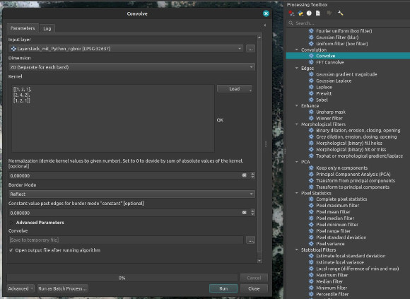
Neues QGIS-Plugin für Rasterlayer mit Faltung, morphologischen Filtern, Hauptkomponentenanalyse, Statistik etc.
Mein neues QGIS-Plugin Scipy Filters ermöglicht es, Raster-Layer mithilfe von Scipy zu verarbeiten. Dies ist eine Python-Bibliothek mit einer großen Anzahl an optimierten Algorithmen u.a. für multidimensionale Bildbearbeitung und Signalverarbeitung, die zum Teil bei der Analyse von Rasterdaten nützlich sein können.
Auf die Idee bin ich gekommen, weil in der neusten QGIS-Version die Orfeo-Toolbox abgeschafft wurde und ich damit keine morphologischen Filter mehr hatte. Es war früher ziemlich umständlich, die Orfeo-Toolbox zu installieren, und ein Plugin, das Scipy verwendet, schien mir die beste Alternative. Letztlich habe ich es so programmiert, dass mit relativ wenig Aufwand eine große Zahl an Filtern bereitgestellt werden kann — so viele, dass sie in der Processing-Toolbox auf meinem Monitor nicht alle gleichzeitig angezeigt werden.
In den meisten Fällen stellt mein Plugin das User Interface bereit, reicht die Rasterdaten an die jeweilige Scipy-Funktion weiter und lädt das Ergebnis wieder in QGIS. Ich habe auch ein paar zusätzliche Filter geschrieben, die es nicht direkt in Scipy gibt: Insbesondere die Hauptkomponentenanalyse (PCA), implementiert mithilfe von Single Value Decomposition (SVD).
Viele der Filter arbeiten innerhalb einer individuell definierbaren Nachbarschaft, in der z.B. der lokale Mittelwert, Standardabweichung etc. berechnet werden kann. Neben klassischen Weichzeichnern und Kantenerkennung (Sobel, Laplace etc.) gibt es auch Faltung mit einem benutzerdefinierten Kernel.