Update: For an improved version see my jupyter notebook.
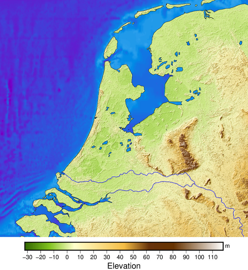
With Python and PyGMT it is quite easy to draw a simple topo map based on NASA elevation data (public domain!). However, the simplest approach relies on a colormap colouring everything below 0 m mean sea level in shades of blue, everything above 0 m in shades of green/brown (e.g. with cmap=”geo”). With a world map or in the mountains the result looks pretty good, but with coastlines on detailed maps there are problems. A map of Holland clearly shows the problem:
import pygmt
region=[3.2, 6.8, 51.4, 53.5]
grid = pygmt.datasets.load_earth_relief(resolution="03s",
       region=region)

fig = pygmt.Figure()
fig.grdimage(grid=grid, projection="M15c", cmap="geo")
fig.colorbar(frame=["a10", "x+lElevation", "y+lm"])
fig.coast(shorelines=True, region=region, resolution="f")
fig.show()
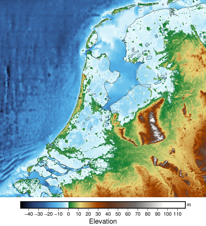
It shows half of Holland under water … I did not find any instructions in the tutorials and docs on how to solve the problem. But with the help of pygmt.grdlandmask it was quite simple. This approach is based on the coastline used in fig.coast(). The generated mask sets the value specified for “dry” or “wet” (e.g. 0 or 1) for each pixel. The first trick is that this mask can simply be multiplied by the grid, then all water pixels are set to 0. Now we can draw the land with a suitable colormap, e.g. cmap=”dem1″. As “spacing” for the mask I use the value of the “resolution” of the dataset and “resolution” of the mask is “f”, i.e. full resolution as in fig.coast().
(Update: With pygmt 0.9 and later, it is possible to download a mask grid with pygmt.datasets.load_earth_mask instead of calculating it with pygmt.grdlandmask.)
We plot the water over the result in the second step. However, we cannot simply use “maskvalues=[1, 0]” now, because then the land becomes shallow water of 0 m depth. Fortunately, it is possible to specify “NaN” (as a string) as a value in the mask. And in fig.grdimage we can ensure with “nan_transparent=True” that the land is now transparent.
land = grid * pygmt.grdlandmask(region=region,
     spacing="03s",
     maskvalues=[0, 1],
     resolution="f")
wet = grid * pygmt.grdlandmask(region=region,
     spacing="03s",
     maskvalues=[1, "NaN"],
     resolution="f")

fig = pygmt.Figure()

# Plot land (with hill shading)
fig.grdimage(grid=land, projection="M15c",
     cmap="dem1", shading=True)
fig.colorbar(frame=["a10", "x+lElevation", "y+lm"])

# Plot water (NaN transparent)
fig.grdimage(grid=wet,
     cmap="seafloor", nan_transparent=True)

fig.coast(shorelines=True, projection="M15c",
     region=region, resolution="f")
fig.coast(rivers="1/0.5p,blue") # Rivers

fig.show()