With PyGMT it is quite easy to plot good looking maps. As an example, I show how to create a simple trekking map of the Tour du Mont Blanc. In detail, the syntax is a bit esoteric, it goes back to the syntax of the General Mapping Tool (see PyGMT’s docs).
import pygmt
import geopandas as gpd
import pandas as pd
If the entire GPS track is a single file, we can read it into a GeoDataFrame with the following command. If there are many files, see Open GPS tracks (GPX files) with Geopandas.
track = gpd.read_file('gpx/tmb.gpx', layer='tracks')
We can get a first impression of the track with track.plot(), and track.total_bounds returns min and max values of latitude and longitude.
With pygmt.datasets.load_earth_relief we get the topo data (gathered by NASA) from the web. For this scale resolution="01s" (i.e. 1 arc second) is suitable, for overview maps (regions, continents, world) it is essential to choose a different resolution. The topo data can be plotted with grdimage. The function “coast” can draw not only coasts, but also large rivers and borders. The function “plot” draws the geometry of the track.
lat_min, long_min, lat_max, long_max = track.total_bounds

# Add some margin
lat_min -= 0.1
lat_max += 0.1
long_max += 0.06
long_min -= 0.05

region = [lat_min, lat_max, long_min, long_max]

grid = pygmt.datasets.load_earth_relief(resolution="01s", region=region)

fig = pygmt.Figure()
fig.grdimage(grid=grid, projection="M15c", cmap="dem2", shading=True)
#fig.colorbar(frame=["a1000", "x+lElevation", "y+lm"])

# Plot borders
fig.coast(borders=["1/0.5p,red,..-"], resolution="f")

# Plot track
fig.plot(data=track, pen="1.5p,white")
fig.plot(data=track, pen="0.8p,blue")
fig.show()
Now our map already looks quite good, but the towns and important peaks are still missing. I’ll start with a simple list and try to get the coordinates by geocoding.
peaks_list = [ 'Mont Blanc', 'Grandes Jorasses', 'Mont Dolent']
towns_list = ['Chamonix', 'Les Houches', 'Les Contamines', 'Courmayeur', 'Praz de Fort', 'Champex', 'Martigny']

# Get coordinates with gpd.tools.geocode
# (requires GeoPy)

peaks = gpd.tools.geocode(peaks_list)
peaks['label'] = peaks_list

towns = gpd.tools.geocode(towns_list)
towns['label'] = towns_list
Using the code below, these locations can be plotted over the map. However, the town Les Contamines was not visible on the map because the coordinates returned by geocode were not correct. I prepare another geodataframe with a list and attach it. I also define additional “places”.
correct_towns = [['Les Contamines', 45.822746, 6.726553]]

correct_towns = pd.DataFrame(correct_towns, columns = ['label', 'latitude', 'longitude'])
correct_towns = gpd.GeoDataFrame(
    correct_towns, geometry=gpd.points_from_xy(correct_towns.longitude, correct_towns.latitude))

towns = towns.append(correct_towns)

# These places did not get usable coordinates
# with geocoding
# and I also want different markers
places = [['Col de la Forclaz', 46.059, 7.0022],
         ['Flégère', 45.9604, 6.8865]]

places = pd.DataFrame(places, columns = ['label', 'latitude', 'longitude'])
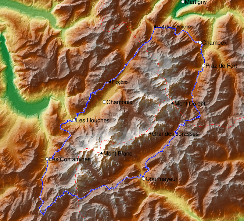
Now we can complete the map. With “plot” we draw different markers for cities, peaks and other places; “text” writes the label next to it (x with a small margin).
fig.plot(data=towns, style="c0.2c", color="white", pen="black")
fig.text(text=towns.label, x=towns.geometry.x + 0.005, y=towns.geometry.y, justify="ML", font="10p")

fig.plot(x=places.longitude, y=places.latitude, style="c0.15c", color="black")
fig.text(text=places.label, x=places.longitude + 0.005, y=places.latitude, justify="ML", font="8p")

fig.plot(data=peaks, style="t0.2c", color="black")
fig.text(text=peaks.label, x=peaks.geometry.x + 0.005, y=peaks.geometry.y, justify="ML", font="10p")

fig.show()
Unfortunately, the topo data is not always completely error-free, with virtual peaks and holes. And the coasts of lakes are quite inaccurate at this scale. I therefore gave up the idea of drawing a map of the Torres del Paine Cirquit.