Unfortunately, simple GPS devices are quite inaccurate when it comes to elevation. The vertical error is about ± 15 m with a good GPS signal and unobstructed view of the sky. This makes the measured elevation useless for a profile along a GPS track. Some tracking apps like runkeeper get around the problem by sending each point to a web service that returns the altitude “from the map” instead of using measured elevation (see also: Explore runkeeper GPS tracks with python, part 1 and part 2). However, anyone who wants to replace inaccurate elevation data in a GPX file (or assign missing elevation) can easily do so with Python. Based on the freely available SRTM data, we can easily determine the elevation of our points and save the result as a GPX file.
The SRTM data were measured by radar from a space shuttle. The module elevation downloads the SRTM data of our region from the web, and from the individual tiles it creates a single file. This is a geotiff, basically a TIF image with georeference in the metadata. It has (like a greyscale image) only one channel and the value of each pixel is the elevation in metres. The resolution of the file is 1 arcsecond, i.e. about 1 pixel every 30 m. We can open the Geotiff (our digital elevation model, DEM) with rasterio and use it to sample the values at individual coordinates.
Some preparation
import pandas as pd
import geopandas as gpd
import numpy as np
import os
import elevation
import rasterio

track_in = 'gpx/2021-05-22-163014.gpx'
track_out = 'test.gpx'

dem_file = '2021-05-22-163014.tif'
demfolder = "dem" # Where to save the DEM
Open the GPX track with Geopandas
We can simply use Geopandas to open the GPX file (see also this post).
gdf = gpd.read_file(track_in, layer='track_points')
This command uses GDAL under the hood. With layer='track_points' we simply get all the trackpoints of the track, to get waypoints use layer='waypoints' instead.
GDAL returns a lot of useless columns with “None” values, we can drop them. And time should be in datetime (important if we want to save our GPS track as GPX).
gdf.dropna(axis=1, inplace=True)
gdf['time'] = pd.to_datetime(gdf['time'])

gdf.head()
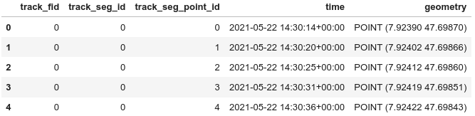
Note the columns ‘track_fid’ and ‘track_seg_id’: They are used by GDAL to reference different tracks and track segments eventually contained in the GPX file. You won’t find these id values if you open the GPX file in a text editor. However it is important to keep these columns to be able to save the track back into a GPX file.
We also need the bounds of our region. I add some margin to be able to use the DEM for other tasks in the region.
# Get the bounds of the track
minx, miny, maxx, maxy = gdf.dissolve().bounds.loc[0]

# You might want to add some margin if you want to use the DEM for other tracks/tasks
minx, miny, maxx, maxy = bounds  = minx - .05, miny - .05, maxx + .05, maxy + .05
Get the DEM with elevation
# Make sure the dem folder does exist
# (otherwise the module elevation fails)
if not os.path.exists(demfolder):
    os.mkdir(demfolder)

# And use an absolute path,
# the module elevation does not work with relative paths.
dem_file = os.path.join(os.getcwd(), demfolder, dem_file)

# Download DEM
elevation.clip(bounds=bounds, output=dem_file)

# Clean temporary files
elevation.clean()
Open and sample the DEM with rasterio
Open the file with rasterio and load the data of the first (and only) channel into a numpy array:
dem_data = rasterio.open(dem_file)
dem_array = dem_data.read(1)
Note: Our DEM already uses the same CRS as our GPS data (WGS84 = EPSG 4326), we don’t need to reproject. You might want to check CRS and size of the DEM with dem_data.crs, dem_data.width, dem_data.height, get the bounds with dem_data.bounds and the amount of channels with dem_data.count.
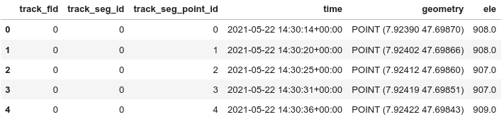
All the magic is happening in the next line: dem_data.index() takes the coordinates (longitude, latitude) and returns the index values of our array. We can use these index values to get the value from the array. Note: GPX uses the tag <ele> </ele> for elevation, ‘ele’ must be the column name. And we get an int, but it must be float to save the GeoDataFrame as GPX file.
gdf['ele'] = dem_array[dem_data.index(gdf['geometry'].x, gdf['geometry'].y)]

# Note that we get ele values as int.
# To save as GPX, ele must be as float.
gdf['ele'] = gdf['ele'].astype(float)

gdf.head()
Of course, our data is still in increments of 1 meter and a profile looks correspondingly stepped (see below). I compared the result to the elevation of runkeeper tracks: it comes pretty close. I guess they are using the SRTM data as well, but use interpolation (and a slight blur?) to get a DEM with higher resolution and a smoother profile along the track. We can do this as well, see below. But let’s first save our data to a GPX file.
Save GeoDataFrame as GPX
Geopandas makes it very easy to save our GeoDataFrame as GPX file (note: I defined the filename track_out at the start):
gdf.to_file(track_out, 'GPX', layer='track_points')
Important: This fails if the file already exists! You’ll need to delete an existing file first.
Use layer='waypoints' if you were working with waypoints. (Remember that time must be in datetime and to save the points as track we need ‘track_fid’ and ‘track_seg_id’.)
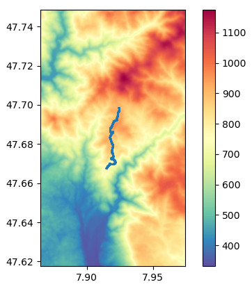
Extra: Have a look at the DEM
We can also have a quick look at our DEM. Turn the DEM into a map and plot the track:
import matplotlib.pyplot as plt

vmin = dem_array.min()
vmax = dem_array.max()
extent = minx, maxx, miny, maxy

fig, ax = plt.subplots()
cax = plt.imshow(dem_array, extent=extent,
                  cmap='Spectral_r', vmin=vmin, vmax=vmax)
fig.colorbar(cax, ax=ax)
gdf.plot(ax=ax, markersize=1, zorder=11)
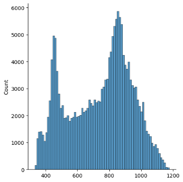
And a histplot of elevations:
import seaborn as sns
sns.displot(dem_array.ravel())
Smooth and upscale the DEM
To get a smoother profile along the track, we can smooth and upscale our DEM. Note: The upscaled data is not necessarily more accurate. First we have to cast our array to float. Then we can apply a slight gaussian blur to smooth out the steps in the terrain. Of course, the rounded values should still be the same as the original int values (sigma=0.33 works fine for my example, you might want to adjust it).
dem_array_float = dem_array.astype(float)

from scipy import ndimage

# Blur to reduce the steps in the DEM.
# With sigma 0.33 I am still very close to the original.
dem_array_float = ndimage.gaussian_filter(dem_array_float, sigma=0.33)
Now we can upscale our array to get a pixel for every few meters. Note: scipy.ndimage.zoom() resamples with cubic interpolation with order=3 (the default). We also need a new transform matrix. It will be used by rasterio to map coordinates (latitude, longitude) to pixel indices.
upscale_factor = 5

# Upscale the array
dem_array_float = ndimage.zoom(dem_array_float, upscale_factor).round(decimals=1)


# Scale the transform matrix
transform = dem_data.transform * dem_data.transform.scale(
        (dem_data.width / dem_array_float.shape[-1]),
        (dem_data.height / dem_array_float.shape[-2])
    )
Now we are ready to sample the elevation data for our track points:
gdf['ele_resample'] = dem_array_float[rasterio.transform.rowcol(transform, gdf['geometry'].x, gdf['geometry'].y)]
We can plot a profile (after calculating the distance along the track):
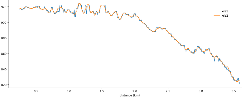
The figure zooms into a part of my track: blue using elevation of the original DEM with int values, orange using the smoothed and upscaled DEM. Since I used a runkeeper track, I can calculate the difference of my models with the elevation reported by runkeeper. Using describe() I get:
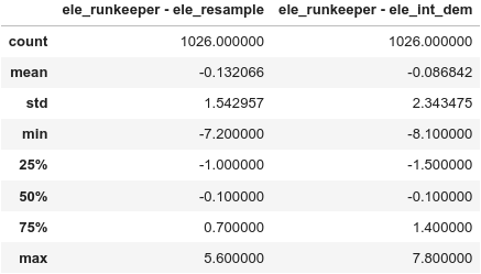
Using the upscaled DEM, my elevation is within ± 1 m of the value reported by runkeeper for more than 50 % of all trackpoints. Pretty impressive! There are some outliers, but I don’t know which model is closer to the real terrain.