In part 1 of this series, I explored a single GPS track with geopandas and folium. The next step is to wrap the code preparing the GeoDataFrame into a function. Then I read all GPX files of a given folder and run my function on these tracks.
Function to prepare GeoDataFrames
After importing some modules and setting the file path, I define a function that does pretty much the same as my part 1. I added code to handle weird outliers: After pauses/stops (i.e. waiting at a traffic light), the GPS used by runkeeper sometimes was a bit confused and didn’t really know where I was. In one case, the first point after a stop was 1.6 km away from the real position, resulting in one line segment with a speed of more than 400 km/h — and a total distance that was 3.3 km too long.
import pandas as pd
import geopandas as gpd
import numpy as np
import os
from shapely.geometry import LineString
import folium

folder = "gpx/"

def prepare_dataframes(gdf, track_name):
    """ Calculate distance, speed etc. from raw data of gpx trackpoints.
    Return two GeoDataframes: points and (connecting) lines.
    """
    gdf.index.names = ['point_id']
    gdf['time'] = pd.to_datetime(gdf['time'])
    gdf.dropna(axis=1, inplace=True)
    gdf.drop(columns=['track_fid', 'track_seg_id', 'track_seg_point_id'], inplace=True)

    # Use local UTM to get geometry in meters
    gdf = gdf.to_crs(gdf.estimate_utm_crs())

    # shifted gdf gives us the next point with the same index
    # allows calculations without the need of a loop
    shifted_gdf = gdf.shift(-1)

    gdf['time_delta'] = shifted_gdf['time'] - gdf['time']
    gdf['time_delta_s'] = gdf['time_delta'].dt.seconds
    gdf['dist_delta'] = gdf.distance(shifted_gdf)

    # In one track, after making a pause, I had a weird outlier 1.6 km away of my real position.
    # Therefore I replace dist_delta > 100 m with NAN.
    # This should be counted as pause.
    gdf['dist_delta'] = np.where(gdf['dist_delta']>100, np.nan, gdf['dist_delta'])

    # speed in various formats
    gdf['m_per_s'] = gdf['dist_delta'] / gdf.time_delta.dt.seconds
    gdf['km_per_h'] = gdf['m_per_s'] * 3.6
    gdf['min_per_km'] = 60 / (gdf['km_per_h'])

    # We now might have speeds with NAN (pauses, see above)
    # Fill NAN with 0 for easy filtering of pauses
    gdf['km_per_h'].fillna(0)


    # covered distance (meters) and time passed
    gdf['distance'] = gdf['dist_delta'].cumsum()
    gdf['time_passed'] = gdf['time_delta'].cumsum()

    # Minutes instead datetime might be useful
    gdf['minutes'] = gdf['time_passed'].dt.seconds / 60

    # Splits (in km) might be usefull for grouping
    gdf['splits'] = gdf['distance'] // 1000

    # ascent is = elevation delta, but only positive values
    gdf['ele_delta'] = shifted_gdf['ele'] - gdf['ele']
    gdf['ascent'] = gdf['ele_delta']
    gdf.loc[gdf.ascent < 0, ['ascent']] = 0

    # Slope in %
    gdf['slope'] = 100 * gdf['ele_delta'] / gdf['dist_delta']

    # slope and min_per_km can be infinite if 0 km/h
    # Replace inf with nan for better plotting
    gdf.replace(np.inf, np.nan, inplace=True)
    gdf.replace(-np.inf, np.nan, inplace=True)

    # Ele normalized: Startpoint as 0
    gdf['ele_normalized'] = gdf['ele'] - gdf.loc[0]['ele']

    # Back to WGS84 (we might have tracks from different places)
    gdf = gdf.to_crs(epsg = 4326)
    shifted_gdf = shifted_gdf.to_crs(epsg = 4326)

    # Create another geodataframe with lines instead of points as geometry.
    lines = gdf.iloc[:-1].copy() # Drop the last row
    lines['next_point'] =  shifted_gdf['geometry']
    lines['line_segment'] = lines.apply(lambda row:
        LineString([row['geometry'], row['next_point']]), axis=1)
    lines.set_geometry('line_segment', inplace=True, drop=True)
    lines.drop(columns='next_point', inplace=True)
    lines.index.names = ['segment_id']

    # Add track name and use it for multiindex
    gdf['track_name'] = track_name
    lines['track_name'] = track_name
    gdf.reset_index(inplace=True)
    gdf.set_index(['track_name', 'point_id'], inplace=True)
    lines.reset_index(inplace=True)
    lines.set_index(['track_name', 'segment_id'], inplace=True)
    return gdf, lines
Now we can open the GPX files and populate our GeoDataFrames with data.
# Prepare empty Geodataframes
points = gpd.GeoDataFrame()
lines = gpd.GeoDataFrame()

# And populate them with data from gpx files
for file in os.listdir(folder):
    if file.endswith(('.gpx')):
        try:
            rawdata = gpd.read_file(folder + file, layer='track_points')
            track_points, track_lines = prepare_dataframes(rawdata, file)
            points = pd.concat([points, track_points])
            lines = pd.concat([lines, track_lines])
        except:
            print("Error", file)
lines.head()
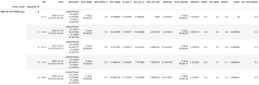
How comparable are line segments?
Simple plots would be more meaningful if each line segment has a similar length in time or distance. My conclusion after examining different plots of 'dist_delta', 'time_delta' and speed: The sampling frequency is usually one point every 3 to 6 seconds. Runkeeper seems to change the sampling frequency according to current speed and gets pretty regular distances between sampling points (one point every 9 to 12 m). The exception are segments with very low speeds of 0 to 1.5 km/h, i.e. pauses. I think this makes line segments comparable enough to use them for simple plots, we can assume every segment to be approx 10 m or a pause. We could think about filtering out segments with very low speeds.
Note that I sometimes have absurd high speeds, when the GPS signal was not accurate. This happened below bridges or right after a pause/stop. We can filter them out as well.
Basic statistics
With a few lines of code we can get some basic statistics of our tracks. Try the following:
Ascent in meters:
lines.groupby('track_name')['ascent'].sum()
Try also:
lines.groupby('track_name')['ascent'].sum().describe()
Distance in meters:
lines.groupby('track_name')['distance'].sum().describe()
Speed:
lines.groupby('track_name')['km_per_h'].describe()
Extract some useful information about each run
I create a pandas Dataframe with general information about each run, such as distance, ascent, mean speed. I also calculate the time of pauses (all intervals with very low speed, I set the threshold as 1.5 km/h).
runs = pd.DataFrame({
              'distance': lines.groupby('track_name')['dist_delta'].sum(),
              'ascent': lines.groupby('track_name')['ascent'].sum(),
              'start_time': points.groupby('track_name')['time'].min(),
              'end_time': points.groupby('track_name')['time'].max(),
              'median_km_h' : lines.groupby('track_name')['km_per_h'].median()
              })

runs['total_duration'] = runs['end_time'] - runs['start_time']

# Pauses (speed <1.5 km/h)
runs['pause'] = lines[
      lines['km_per_h']<1.5
      ].groupby('track_name')['time_delta'].sum()
runs['pause'] = runs['pause'].fillna(pd.Timedelta(0))

# Duration without pauses
runs['duration'] = runs['total_duration'] - runs['pause']
runs['minutes'] = runs.duration.dt.seconds / 60

# Speed
runs['m_per_s'] = runs['distance'] / runs.duration.dt.seconds
runs['km_per_h'] = runs['m_per_s'] * 3.6
runs['min_per_km'] = 60 / runs['km_per_h']

# Distance in km
runs['distance'] = runs['distance'] / 1000
You can also turn runs into a GeoDataFrame and add the geometry of the complete track:
# Add Geometry of the (complete) runs
runs = gpd.GeoDataFrame(runs, geometry=lines.dissolve(by='track_name')['geometry'])
For some statistics, try:
runs.describe()
Some Queries
You may want to find the fastest or longest run or similar information.
To get the 5 longest runs:
runs.sort_values(by='distance', ascending=False).head(5)
The 5 fastest runs:
runs.sort_values(by='km_per_h', ascending=False).head(5)
Fastest runs in the range from 8 to 12 km:
runs[(runs['distance']>=8) & (runs['distance']<=12)].sort_values(by='km_per_h', ascending=False).head(5)
Reports per month and per year
How many activities did I have last year? What was the total distance covered in March? We can create a table to answer such questions.
Report per year:
per_year = pd.DataFrame({
              'count': runs.groupby(runs.start_time.dt.year)['distance'].count(),
              'total_distance': runs.groupby(runs.start_time.dt.year)['distance'].sum(),
              'distance_median': runs.groupby(runs.start_time.dt.year)['distance'].median(),
              'distance_mean': runs.groupby(runs.start_time.dt.year)['distance'].mean(),
              'distance_max': runs.groupby(runs.start_time.dt.year)['distance'].max(),
              'total_ascent': runs.groupby(runs.start_time.dt.year)['ascent'].sum(),
              'ascent_median': runs.groupby(runs.start_time.dt.year)['ascent'].sum(),
              'ascent_max': runs.groupby(runs.start_time.dt.year)['ascent'].max(),
              'median_km_h' : runs.groupby(runs.start_time.dt.year)['km_per_h'].median(),
              'mean_km_h' : runs.groupby(runs.start_time.dt.year)['km_per_h'].mean(),
              })

per_year.index.name = 'year'

per_year
And a report per month:
per_month = pd.DataFrame({
              'count': runs.groupby([runs.start_time.dt.year,
                                     runs.start_time.dt.month])['distance'].count(),
              'total_distance': runs.groupby([runs.start_time.dt.year,
                                    runs.start_time.dt.month])['distance'].sum(),
              'distance_median': runs.groupby([runs.start_time.dt.year,
                                    runs.start_time.dt.month])['distance'].median(),
              'distance_mean': runs.groupby([runs.start_time.dt.year,
                                    runs.start_time.dt.month])['distance'].mean(),
              'distance_max': runs.groupby([runs.start_time.dt.year,
                                    runs.start_time.dt.month])['distance'].max(),
              'total_ascent': runs.groupby([runs.start_time.dt.year,
                                    runs.start_time.dt.month])['ascent'].sum(),
              'ascent_median': runs.groupby([runs.start_time.dt.year,
                                    runs.start_time.dt.month])['ascent'].sum(),
              'ascent_max': runs.groupby([runs.start_time.dt.year,
                                    runs.start_time.dt.month])['ascent'].max(),
              'median_km_h' : runs.groupby([runs.start_time.dt.year,
                                    runs.start_time.dt.month])['km_per_h'].median(),
              'mean_km_h' : runs.groupby([runs.start_time.dt.year,
                                    runs.start_time.dt.month])['km_per_h'].mean(),
              })

per_month.index.names = ['year', 'month']

per_month
The following alternative way also shows months with zero activity (useful for plotting):
freq = runs.set_index('start_time').groupby(pd.Grouper(freq="M"))

freq_month = pd.DataFrame({
              'count': freq['distance'].count(),
              'total_distance': freq['distance'].sum(),
              'distance_median': freq['distance'].median(),
              'distance_mean': freq['distance'].mean(),
              'distance_max': freq['distance'].max(),
              'total_ascent': freq['ascent'].sum(),
              'ascent_median': freq['ascent'].sum(),
              'ascent_max': freq['ascent'].max(),
              'median_km_h' : freq['km_per_h'].median(),
              'mean_km_h' : freq['km_per_h'].mean(),
              })

freq_month.index.name = 'month_dt'
freq_month['year'] = freq_month.index.year
freq_month['month'] = freq_month.index.month

freq_month
Plot: freq_month['count'].plot(kind='bar')
Plots with seaborn
Now it is time for your visualisation skills. In this post I only show some examples, you find many more in the jupyter notebook.
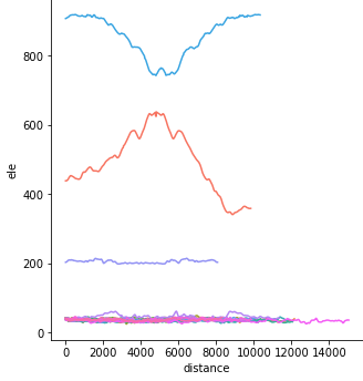
Profiles of the tracks:
sns.relplot(x="distance", y="ele", data=lines, kind="line", hue="track_name");
You can also try a normalised version, with all tracks starting at zero:
sns.relplot(x="distance", y="ele_normalized", data=lines, kind="line", hue="track_name");
Does speed relate to slope? (Note that I filter out unrealistic high speeds)
sns.relplot(x="slope", y="km_per_h", data=lines[lines['km_per_h']<30], hue="track_name");
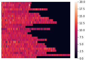
Let's plot a heatmap of speed.
heatmapdata1 = lines.reset_index()
heatmapdata1 = heatmapdata1.pivot(index='track_name', columns='segment_id', values='km_per_h')
heatmapdata1.fillna(value=0, inplace=True)

# Set vmax to filter out unrealistic values
sns.heatmap(heatmapdata1, vmin=0, vmax=20, xticklabels=False)
A heatmap of ele_delta is interesting as well. I set minimum and maximum values, otherwise the result is almost completely black.
heatmapdata2 = lines.reset_index()
heatmapdata2 = heatmapdata2.pivot(index='track_name', columns='segment_id', values='ele_delta')
heatmapdata2.fillna(value=0, inplace=True)
sns.heatmap(heatmapdata2, xticklabels=False, center=0, vmin=-2, vmax=2)
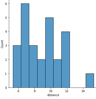
A histogram of the distance of the tracks:
sns.displot(x="distance", data=runs, binwidth=1);
You should try also speed vs. distance
sns.relplot(x="distance", y="km_per_h", data=runs, hue="track_name")
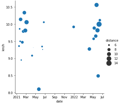
Speed (and distance) vs. date:
import matplotlib.dates as mdates

g = sns.relplot(x="start_time", y="km_per_h", data=runs, size="distance", sizes=(2,300))
g.ax.set_xlabel("date")
g.ax.set_ylabel("km/h")
g.ax.xaxis.set_major_formatter(
    mdates.ConciseDateFormatter(g.ax.xaxis.get_major_locator()))
and:
g = sns.relplot(x="start_time", y="distance", data=runs, size="km_per_h")
g.ax.set_xlabel("date")
g.ax.set_ylabel("distance")
g.ax.xaxis.set_major_formatter(
    mdates.ConciseDateFormatter(g.ax.xaxis.get_major_locator()))
Distance vs. minutes:
sns.jointplot(x="distance", y="minutes", data=runs, kind="reg")
You can also plot your monthly reports. For nicer plots, I replace year and month with a datetime index.
per_month_dt = per_month.reset_index()
per_month_dt['month'] =  pd.to_datetime(per_month_dt['year'].astype('str') + '-' + per_month_dt['month'].astype('str') + '-1')
per_month_dt.drop(columns='year', inplace=True)
per_month_dt.set_index('month', inplace=True)
And now you can plot the monthly total distance:
g = sns.relplot(x="month", y="total_distance", data=per_month_dt)
g.ax.xaxis.set_major_formatter(
    mdates.ConciseDateFormatter(g.ax.xaxis.get_major_locator()))
Or the median of speed for each month:
g = sns.relplot(x="month", y="median_km_h", data=per_month_dt)
g.ax.xaxis.set_major_formatter(
    mdates.ConciseDateFormatter(g.ax.xaxis.get_major_locator()))
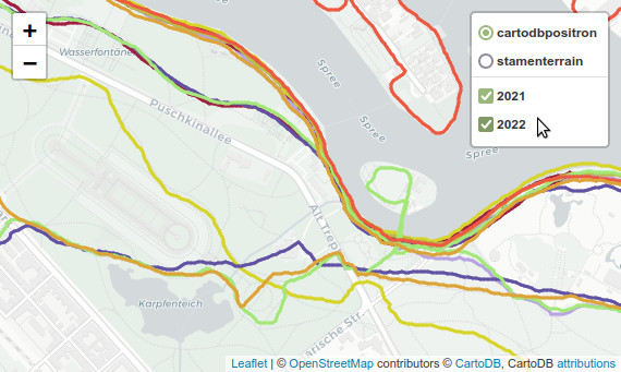
Interactive map with Folium
Finally we can use folium to plot all tracks on a interactive map (see screenshot at the start of my post). The map has tooltips, showing the actual speed, kilometer, time etc. of each line segment. The tracks of every year can be switched on and off, and you can choose one of two different base maps.
For meaningfull tooltips I have to plot the actual line segments instead of the complete runs. First, I create a cleaned up GeoDataFrame without datetime (otherwise folium fails), and with rounded values (for nicer tooltips).
lines_condensed = lines[['ele_delta', 'dist_delta', 'geometry', 'distance', 'km_per_h', 'min_per_km', 'minutes', 'slope', 'time_delta_s']].dropna().copy()

lines_condensed['date'] = lines['time'].dt.strftime("%d %B %Y")
lines_condensed['year'] = lines['time'].dt.year
lines_condensed['month'] = lines['time'].dt.month

lines_condensed.reset_index(level=1, inplace=True)
lines_condensed['total_distance'] = runs['distance']
lines_condensed['total_minutes'] = runs['minutes']

lines_condensed['distance'] = lines_condensed['distance']/1000
lines_condensed['distance'] = lines_condensed['distance'].round(2)
lines_condensed['total_distance'] = lines_condensed['total_distance'].round(2)
lines_condensed['total_minutes'] = lines_condensed['total_minutes'].round(2)
lines_condensed['minutes'] = lines_condensed['minutes'].round(2)
lines_condensed['min_per_km'] = lines_condensed['min_per_km'].round(2)
lines_condensed['km_per_h'] = lines_condensed['km_per_h'].round(2)
lines_condensed['slope'] = lines_condensed['slope'].round(3)
We need a style function and I assign a random color to each track.
# style function
def style(feature):
        return {
            # 'fillColor': feature['properties']['color'],
            'color': feature['properties']['color'],
            'weight': 3,
        }


for x in lines_condensed.index:
    color = np.random.randint(16, 256, size=3)
    color = [str(hex(i))[2:] for i in color]
    color = '#'+''.join(color).upper()
    lines_condensed.at[x, 'color'] = color
I use the last (youngest) location as map location.
location_x = lines_condensed.iloc[-1]['geometry'].coords.xy[0][0]
location_y = lines_condensed.iloc[-1]['geometry'].coords.xy[1][0]
Group by year:
grouped = lines_condensed.groupby('year')
And finally plot the map. (I explained the feature groups here.)
m = folium.Map(location=[location_y, location_x], zoom_start=13, tiles='cartodbpositron')
folium.TileLayer('Stamen Terrain').add_to(m)

# Iterate through the grouped dataframe
# Populate a list of feature groups
# Add the tracks to the feature groups
# And add the feature groups to the map

f_groups = []

for group_name, group_data in grouped:
    f_groups.append(folium.FeatureGroup(group_name))
    track_geojson = folium.GeoJson(data=group_data, style_function=style).add_to(f_groups[-1])
    track_geojson.add_child(
          folium.features.GeoJsonTooltip(fields=['date', 'distance', 'total_distance', 'minutes', 'total_minutes', 'min_per_km', 'km_per_h' ],
                                   aliases=['Date', 'Kilometers', 'Total km', 'Minutes', 'Total min', 'min/km', 'km/h'])
        )
    f_groups[-1].add_to(m)

folium.LayerControl().add_to(m)

m
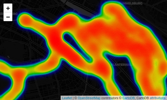
Folium Heatmap
Folium is also very good in plotting interactive heatmaps. The plugin heatmap accapts a list of locations, we can get it from our points GeoDataFrame. You can also play with the parameters, espetially try to adjust radius and blur.
# Create a list of the locations from points
locations = list(zip(points['geometry'].y, points['geometry'].x))

hm = folium.Map(tiles='cartodbdark_matter')

# Add heatmap to map instance
# Available parameters: HeatMap(data, name=None, min_opacity=0.5, max_zoom=18, max_val=1.0, radius=25, blur=15, gradient=None, overlay=True, control=True, show=True)
folium.plugins.HeatMap(locations).add_to(hm)

hm