Fitness tracking apps like runkeeper collect a lot of interesting data. With some python skills, you can have a detailed look at your runs. In the first part of this series I will explore a single GPS track (GPX file) with Python, using Geopandas and Folium. It was inspired by this blog post, but I found a more elegant way without iterating through the GeoDataFrame, and I also add useful tooltips to the map.
In the second part, I change the code in order to get a GeoDataFrame with all my GPS tracks. This is great for plotting and analysing all runs. Part 2 comes with a jupyter notebook, ready to use with your own GPS tracks.
Download the GPS Tracks
To get your runkeeper GPS tracks, log in on https://runkeeper.com/, look for the gear wheel icon, select “Account Settings” and then “Export Data”. You’ll get a ZIP that includes the GPS tracks of your runs as individual GPX files. (When I did this some months ago, I had to wait 2 days before a download link appeard. Last week it worked instantaneously.)
Open the GPX file in Geopandas
Geopandas can open and parse GPX files (using GDAL under the hood). To get a GeoDataFrame with all trackpoints:
import pandas as pd
import geopandas as gpd
import numpy as np
from shapely.geometry import LineString

file = "gpx/2021-01-16-110027.gpx"

gdf = gpd.read_file(file, layer='track_points')
gdf.head()
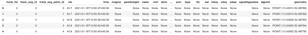
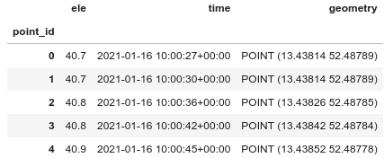
See this post for details about runkeepers elevation data. We can see a lot of columns with “None” values, we can drop them. Note the columns “track_fid”, “track_seg_id” and “track_seg_point_id”: They are used by GDAL to identify different tracks, segments and trackpoints that may be found within a single GPX file. Runkeeper starts a new track segment after a pause, so we can’t simply use track_seg_point_id as index. I will call the index created by Geopandas “point_id” and drop the other columns. The result will include the pauses. I also turn time to Datetime.
# Better use the geodataframe index as point_id
gdf.index.names = ['point_id']
# And turn time to Datetime
gdf['time'] = pd.to_datetime(gdf['time'])

# Drop useless columns
gdf.dropna(axis=1, inplace=True)
gdf.drop(columns=['track_fid', 'track_seg_id', 'track_seg_point_id'], inplace=True)

gdf.head()
Extract information from the track
How long did the run take (including pauses)?
total_time = gdf.iloc[-1]['time'] - gdf.iloc[0]['time']
total_time
Timedelta(‘0 days 00:42:26’)
Now we calculate the distance from point to point. We first have to turn geometry to UTM, to get coordinates in meters instead of degrees. With recent versions of geopandas and pyproj it is easy to estimate the best UTM zone:
gdf = gdf.to_crs(gdf.estimate_utm_crs())
Now I create a second GeoDataFrame with index shifted by -1. This trick makes it easy to compute the distance from one point to the next.
shifted_gdf = gdf.shift(-1)
gdf['time_delta'] = shifted_gdf['time'] - gdf['time']
gdf['dist_delta'] = gdf.distance(shifted_gdf)
Note: The last row of shifted_gdf is populated by NaN values. Therefore we also get NaN as distance for the last row of gdf (from the last trackpoint, there is no distance to the next trackpoint).
Now let’s calculate speed in various formats:
# speed in various formats
gdf['m_per_s'] = gdf['dist_delta'] / gdf.time_delta.dt.seconds
gdf['km_per_h'] = gdf['m_per_s'] * 3.6
gdf['min_per_km'] = 60 / (gdf['km_per_h'])
The covered distance along the track (in meter) and time passed:
gdf['distance'] = gdf['dist_delta'].cumsum()
gdf['time_passed'] = gdf['time_delta'].cumsum()
Additional useful columns:
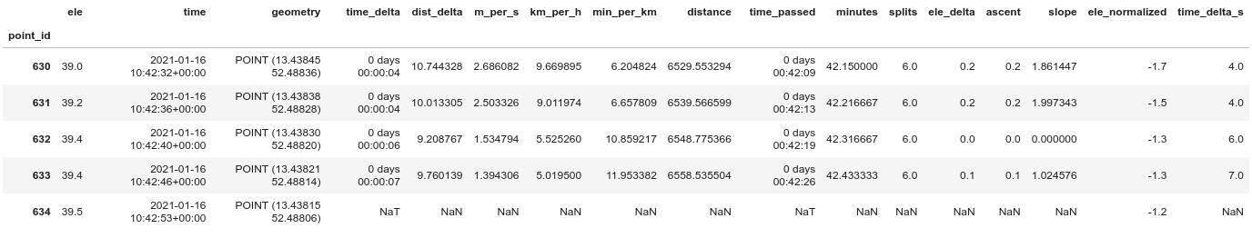
# Minutes instead datetime might be useful
gdf['minutes'] = gdf['time_passed'].dt.seconds / 60

# Splits (in km) might be usefull for grouping
gdf['splits'] = gdf['distance'] // 1000

# ascent is elevation delta, but only positive values
gdf['ele_delta'] = shifted_gdf['ele'] - gdf['ele']
gdf['ascent'] = gdf['ele_delta']
gdf.loc[gdf.ascent < 0, ['ascent']] = 0

# Slope in %
# (since ele_delta is not really comparable)
gdf['slope'] = 100 * gdf['ele_delta'] / gdf['dist_delta']

# Ele normalized: Startpoint as 0
gdf['ele_normalized'] = gdf['ele'] - gdf.loc[0]['ele']

# slope and min_per_km can be infinite if 0 km/h
# Replace inf with nan for better plotting
gdf.replace(np.inf, np.nan, inplace=True)
gdf.replace(-np.inf, np.nan, inplace=True)

# Note the NaNs in the last line
gdf.tail()
Some statistics:
gdf.describe()
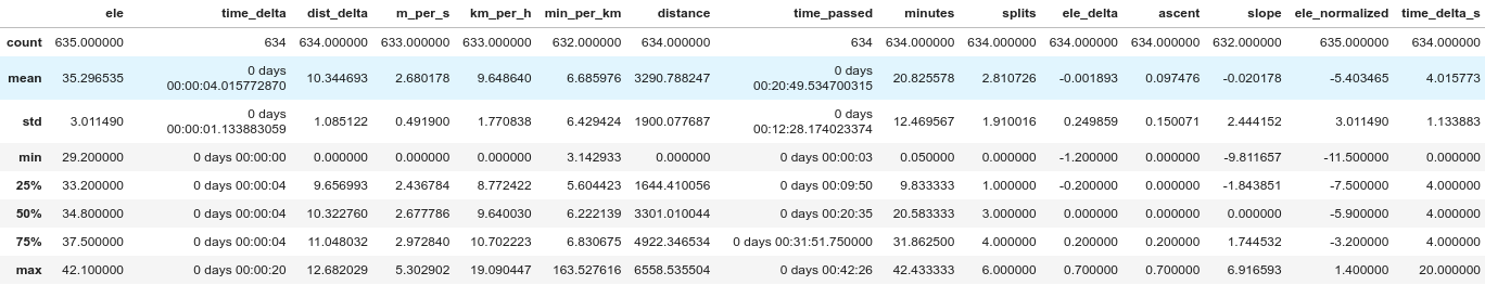
We can get the total ascent (in meters) with:
gdf['ascent'].sum()
We can convert the geometry back to WGS84. This is specially a good idea if you want to compare tracks from different locations (part 2).
gdf = gdf.to_crs(epsg = 4326)
shifted_gdf = shifted_gdf.to_crs(epsg = 4326)
Now it is time for your plotting skills. E.g. a simple profile:
sns.relplot(x="distance", y="ele", data=gdf, kind="line")
plt.ylim(0, 50)
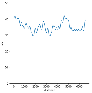
Note: I have set limits for the y-axis, because Berlin is pretty flat and any minor up and down would be greatly exaggerated.
Connect the points with lines
We don't want to plot points on the map, but the lines connecting those points. I create another GeoDataFrame with lines instead of points as geometry. Note that this drops information like time and elevation of the last point. The lambda function uses LineString (module shapely) to create a connecting line. Then we use the line as the new geometry of the GeoDataFrame.
lines = gdf.iloc[:-1].copy() # Drop the last row
lines['next_point'] =  shifted_gdf['geometry']
lines['line_segment'] = lines.apply(lambda row: LineString([row['geometry'], row['next_point']]), axis=1)

lines.set_geometry('line_segment', inplace=True, drop=True)
lines.drop(columns='next_point', inplace=True)
lines.index.names = ['segment_id']
How do the splits compare?
Our column "splits" (segments of 1 km) is handy to compare speed, ascent etc. along the track. Did I get tired in the end? The following code creates a table with a lot of interesting details for each split, like mean, median and standard deviation of speed, ascent and the time needed to complete the split.
lines.groupby('splits').aggregate(
     {'km_per_h': ['mean', 'median', 'max', 'std'],
     'min_per_km': ['mean', 'median', 'max', 'std'],
     'ascent': 'sum',
     'time_delta' : 'sum' })
Map with Folium
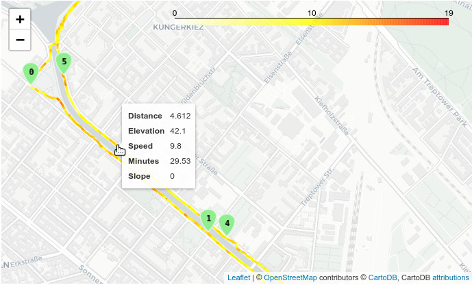
With folium, we can plot an interactive map of our track, including a nice tooltip with information for every line segment (see screenshot at the start of this post).
import folium
import branca.colormap as cm
from folium import plugins

# The approx. center of our map
location = lines.dissolve().convex_hull.centroid
I want to plot markers for each kilometer. We can use the first point of each split.
splitpoints = gdf.groupby('splits').first()
Folium does not like timestamps, drop those columns. And drop rows with speed NaN.
lines_notime = lines.drop(columns=['time', 'time_delta', 'time_passed'] )
lines_notime.dropna(inplace=True)
Round some fields for nicer tooltips
lines_notime['distance'] = (lines_notime['distance']/1000).round(decimals=3)
lines_notime['km_per_h'] = lines_notime['km_per_h'].round(decimals=1)
lines_notime['minutes'] = lines_notime['minutes'].round(decimals=2)
lines_notime['slope'] = lines_notime['slope'].round(decimals=2)
And finally plot the map, using speed for the color. The style function applies color and tooltips to each line segment. For the markers (the "milestones" of the splits) I use folium.plugins.BeautifyIcon, this plugin can plot numbers on the marker.
m = folium.Map(location=[location.y, location.x], zoom_start=15, tiles='cartodbpositron')

# Plot the track, color is speed
max_speed = lines['km_per_h'].max()
linear = cm.LinearColormap(['white', 'yellow', 'red'], vmin=0, vmax=max_speed)
route = folium.GeoJson(
     lines_notime,
     style_function = lambda feature: {
            'color': linear(feature['properties']['km_per_h']),
            'weight': 3},
            tooltip=folium.features.GeoJsonTooltip(
            fields=['distance', 'ele', 'km_per_h', 'minutes', 'slope'],
            aliases=['Distance', 'Elevation', 'Speed', 'Minutes', 'Slope'])
     )

m.add_child(linear)
m.add_child(route)

# Add markers of the splitpoints
for i in range(0,len(splitpoints)):
    folium.Marker(
        location=[splitpoints.iloc[i].geometry.y, splitpoints.iloc[i].geometry.x],
       # popup=str(i),
        icon=plugins.BeautifyIcon(icon="arrow-down",
                                  icon_shape="marker",
                                  number=i,
                                  border_color= 'white',
                                  background_color='lightgreen',
                                  border_width=1)
    ).add_to(m)

m
... and I get the map I showed at the start.
Towards the next step
It's nice to get some statistics for one track. But it would be even nicer to plot the data of all tracks. I will do this in the second part.